RGB	HSI

Python Python Python Python Python

Heidelberg Porcine HyperSPECTRAL Imaging Dataset (HeiPorSPECTRAL)

Welcome to the HeiPorSPECTRAL dataset! Here you can find 5756 hyperspectral imaging (HSI) cubes of 20 physiological organ classes across 11 pigs annotated by 3 medical experts. For each organ, there are about 36 recordings per pig: 4 different intraoperative situations (situs) were imaged from 3 different angles (angle) for 3 times (repetition). The HSI cubes were acquired with the Tivita® Tissue camera system from Diaspective Vision. Each data cube has the dimensions (480, 640, 100) = (height, width, channels) with the 100 non-overlapping spectral channels being in the range from 500 nm to 1000 nm at a spectral resolution of around 5 nm. This repository contains the raw data, related metadata as well as the preprocessed files. The figures from the paper and example visualizations for each image are available at https://figures.heiporspectral.org/.

📝 More details can be found in our publication: Studier-Fischer, A., Seidlitz, S., Sellner, J. et al. HeiPorSPECTRAL - the Heidelberg Porcine HyperSPECTRAL Imaging Dataset of 20 Physiological Organs. Sci Data 10, 414 (2023). https://doi.org/10.1038/s41597-023-02315-8

Interactive visualization for every image.

Interactive figures of the paper. — (Interactive) figures of the paper (including supplementary figures).

Organ profiles aggregated across the entire dataset.

Download

The full dataset can be downloaded at:

https://e130-hyperspectal-tissue-classification.s3.dkfz.de/data/HeiPorSPECTRAL.zip
SHA256: 2152d94f675ee28c2092f675d1b6edca319868c9676b7a71d2c80c1c6fae25ee

Changelog

2023-08-31

Updated HTML files with enhanced navigation bar.
Added preprocessed L1 cubes and parameter images for the colorchecker images.

We do not recommend downloading the archive via the browser due to the large size of 844 GiB. Instead, you may use a download manager of your choice or wget as in the example below. This will allow you to interrupt the download and continue it at a later point. Please make sure beforehand that you have enough free storage to both download the zip archive and decompress the content (around 1.8 TiB). Prior to decompression, it is recommended to verify the checksum of the downloaded file:

# Example for Unix-based systems
# Best to be run in a screen environment (e.g. https://linuxize.com/post/how-to-use-linux-screen/)

# Download all the data
wget --continue https://e130-hyperspectal-tissue-classification.s3.dkfz.de/data/HeiPorSPECTRAL.zip

# Verify the checksum of the downloaded file
curl https://e130-hyperspectal-tissue-classification.s3.dkfz.de/data/HeiPorSPECTRAL.sha256 | sha256sum -c -

An exemplary version of the dataset (ZIP download) is also available for exploring without the need to download the full dataset. It only contains the two images P086#2021_04_15_09_22_02 (spleen) and P093#2021_04_28_08_49_12 (gallbladder).

Usage

We recommend using the data with the htc framework, which offers:

a pipeline to efficiently load and process the HSI cubes, annotations and metadata.
a framework to train neural networks on the data, including the implementation of several classification and segmentation models.
simple usage of pre-trained models.

Installation (example for Unix-based systems):

# Make the dataset available
export PATH_Tivita_HeiPorSPECTRAL=/mnt/nvme_4tb/HeiPorSPECTRAL

# Install the htc package
pip install imsy-htc

As a teaser, this is how you can use the htc framework to read a data cube, corresponding annotation and parameter images:

import numpy as np
from htc import DataPath, LabelMapping

# You can load every image based on its unique name
path = DataPath.from_image_name('P086#2021_04_15_09_22_02')

# HSI cube format: (height, width, channels)
print(path.read_cube().shape)
# (480, 640, 100)

# Annotated region of the selected annotator
mask = path.read_segmentation("polygon#annotator1")
print(mask.shape)
# (480, 640)

# Additional meta information about the image
print(path.meta("label_meta"))
# {'spleen': {'situs': 1, 'angle': 0, 'repetition': 1}}

# Tivita parameter images are available as well
sto2 = path.compute_sto2()
print(sto2.shape)
# (480, 640)

# Example: average StO2 value of the annotated spleen area for annotator1
# The dataset_settings.json file defines the global name to index mapping
spleen_index = LabelMapping.from_path(path).name_to_index("spleen")
print(round(np.mean(sto2[mask == spleen_index]), 2))
# 0.44

Dataset Structure

This dataset contains raw data, annotations, as well as preprocessed data. Annotations were performed by 3 different annotators using a polygon tool. Furthermore, the meta parameters situs, angle and repetition were annotated during image acquisition (see also the JSON Schema file for a meta description of these attributes). Preprocessed data (intermediates) is computed based on the data folder and contains aggregated information and file formats optimized for neural network training. In the following, we explain the structure of this dataset in more detail:

.
├── data/  % Primary animal data (raw data and annotations)
│   ├── subjects/  % Individual animal experiments
│   │   ├── PXXX/  % Folder with all images for this subject (the dataset_settings.json file contains the mapping of the three digit subject identifier used in the dataset to the two digit identifier used in the paper)
│   │   │   ├── YYYY_MM_DD_HH_MM_SS/  % Image data of one recording
│   │   │   │   ├── YYYY_MM_DD_HH_MM_SS_DICOM.dcm  % DICOM file containing the RGB image and parameter images
│   │   │   │   ├── YYYY_MM_DD_HH_MM_SS_meta.log  % Meta information about the recording (e.g. software version, exposure time)
│   │   │   │   ├── YYYY_MM_DD_HH_MM_SS_NIR-Perfusion.png  % NIR perfusion image without background removal
│   │   │   │   ├── YYYY_MM_DD_HH_MM_SS_NIR-Perfusion_segm.png  % NIR perfusion image with background removal
│   │   │   │   ├── YYYY_MM_DD_HH_MM_SS_OHI.png  % Organ Hemoglobin Index (OHI) without background removal
│   │   │   │   ├── YYYY_MM_DD_HH_MM_SS_OHI_segm.png  % Organ Hemoglobin Index (OHI) with background removal
│   │   │   │   ├── YYYY_MM_DD_HH_MM_SS_Oxygenation.png  % Oxygenation (StO2) without background removal
│   │   │   │   ├── YYYY_MM_DD_HH_MM_SS_Oxygenation_segm.png  % Oxygenation (StO2) with background removal
│   │   │   │   ├── YYYY_MM_DD_HH_MM_SS_Parameter.png  % Collage with RGB, StO2, NIR, OHI and TWI images without background removal
│   │   │   │   ├── YYYY_MM_DD_HH_MM_SS_RGB-Image.png  % RGB image
│   │   │   │   ├── YYYY_MM_DD_HH_MM_SS_SpecCube.dat  % Hyperspectral image data cube (float32 binary data of the 30720000 reflectance values)
│   │   │   │   ├── YYYY_MM_DD_HH_MM_SS_THI.png  % Tissue Hemoglobin Index (THI) without background removal
│   │   │   │   ├── YYYY_MM_DD_HH_MM_SS_THI_segm.png  % Tissue Hemoglobin Index (THI) with background removal
│   │   │   │   ├── YYYY_MM_DD_HH_MM_SS_TLI.png  % Tissue Lipid Index (TLI) without background removal
│   │   │   │   ├── YYYY_MM_DD_HH_MM_SS_TLI_segm.png  % Tissue Lipid Index (TLI) with background removal
│   │   │   │   ├── YYYY_MM_DD_HH_MM_SS_TWI.png  % Tissue Water Index (TWI) without background removal
│   │   │   │   ├── YYYY_MM_DD_HH_MM_SS_TWI_segm.png  % Tissue Water Index (TWI) with background removal
│   │   │   │   └── annotations/  % Available annotations for this image
│   │   │   │       ├── YYYY_MM_DD_HH_MM_SS_meta.json  % Structured meta annotation (situs, angle, repetition)
│   │   │   │       ├── YYYY_MM_DD_HH_MM_SS#polygon#annotator1#label#binary.png  % Binary segmentation mask of the polygon from annotator 1 (white = annotated region)
│   │   │   │       ├── YYYY_MM_DD_HH_MM_SS#polygon#annotator1#label#coordinates.csv  % Polygon coordinates for the mask from annotator 1 (col, row)
│   │   │   │       ├── YYYY_MM_DD_HH_MM_SS#polygon#annotator2#label#binary.png  % Binary segmentation mask of the polygon from annotator 2 (white = annotated region)
│   │   │   │       ├── YYYY_MM_DD_HH_MM_SS#polygon#annotator2#label#coordinates.csv  % Polygon coordinates for the mask from annotator 2 (col, row)
│   │   │   │       ├── YYYY_MM_DD_HH_MM_SS#polygon#annotator3#label#binary.png  % Binary segmentation mask of the polygon from annotator 3 (white = annotated region)
│   │   │   │       └── YYYY_MM_DD_HH_MM_SS#polygon#annotator3#label#coordinates.csv  % Polygon coordinates for the mask from annotator 3 (col, row)
│   │   │   └── [more images]
│   │   └── [more subjects]
│   ├── extra_label_symbols/  % Label symbols used in the visualizations as PDF and SVG files
│   │   ├── Cat_01_stomach.pdf
│   │   ├── Cat_01_stomach.svg
│   │   └── [more labels]
│   ├── extra_technical_validation/  % Data for the technical validation (colorchecker measurements)
│   │   ├── Tivita_0202-00118/  % Colorchecker images of the Tivita camera (0202-00118 is the camera ID)
│   │   |   ├── 2022_12_25_colorchecker/  % 13 colorchecker images of the first day
│   │   |   |   ├── YYYY_MM_DD_HH_MM_SS/  % Image data of one recording (similar to the animal data)
│   │   |   |   └── [more images]
│   │   |   └── 2022_12_30_colorchecker/  % 13 colorchecker images of the second day
│   │   |   |   ├── YYYY_MM_DD_HH_MM_SS/
│   │   |   |   └── [more images]
│   │   └── spectrometer/
│   │       └── 2022_09_19_colorchecker/  % Spectrometer measurement data. One file contains the spectra of one color chip (+ white and dark calibrations) at one timestamp with 100 timestamps per measurements
│   ├── dataset_settings.json  % Structured information about the dataset (e.g. label mapping for the blosc segmentations below)
│   └── meta.schema  % JSON Schema defining the structure of the *_meta.json annotation files (possible attributes and types)
│
└── intermediates/ % Processed animal data
    ├── preprocessing/  % Preprocessed files per image
    │   ├── L1/  % L1 normalized data cubes as float16 suitable for network training
    │   │   ├── PXXX#YYYY_MM_DD_HH_MM_SS.blosc  % Compressed binary data
    │   │   └── [more images]
    │   └── parameter_images/  % Tissue parameter images as dictionary of float32 data (StO2, NIR, TWI, OHI, TLI, THI, background)
    │       ├── PXXX#YYYY_MM_DD_HH_MM_SS.blosc  % Dictionary of compressed binary data
    │       └── [more images]
    ├── profiles/  % pdf documents with visualizations comparable to the paper (supplement figure 2+, referred to as profiles), but per image instead of aggregated over the dataset
    │   ├── polygon#annotator1/  % Profile documents for annotator 1
    │   │   ├── polygon#annotator1@01_stomach.pdf  % Profiles for all stomach images of annotator 1
    │   │   └── [more labels]
    │   ├── polygon#annotator2  % Profile documents for annotator 2
    │   └── polygon#annotator3  % Profile documents for annotator 3
    ├── rgb_crops/  % Same RGB images as in the data folder but without the black border (shape 480 x 640)
    │   ├── PXXX/
    │   │   ├── PXXX#YYYY_MM_DD_HH_MM_SS.png
    │   │   └── [more images]
    │   └── [more subjects]
    ├── segmentations/  % Annotation masks per image as dictionary with annotation name as key and label mask as value. The label mask is an np.ndarray of type uint8 and shape 480 x 640. It contains a unique label index for each pixel and combines all available annotations for this image (in case more than one label is annotated). The dataset_settings.json file describes the meaning of the label indices
    │   ├── PXXX#YYYY_MM_DD_HH_MM_SS.blosc
    │   └── [more subjects]
    ├── tables/  % Tables with aggregated data
    │   ├── HeiPorSPECTRAL@median_spectra@polygon#annotator1.csv  % Table with precomputed median spectra (unnormalized, L1-normalized and standard deviation). One row corresponds to a single label of one image annotated by annotator 1. Additional meta information is included as well (e.g. meta information about the recording)
    │   ├── HeiPorSPECTRAL@median_spectra@polygon#annotator1.feather  % Same table as the above CSV file but stored in the feather format (smaller file size and faster to read from within Python)
    │   ├── HeiPorSPECTRAL@median_spectra@polygon#annotator2.csv
    │   ├── HeiPorSPECTRAL@median_spectra@polygon#annotator2.feather
    │   ├── HeiPorSPECTRAL@median_spectra@polygon#annotator3.csv
    │   ├── HeiPorSPECTRAL@median_spectra@polygon#annotator3.feather
    │   ├── HeiPorSPECTRAL@meta.csv
    │   └── HeiPorSPECTRAL@meta.feather  % Structured meta information about an image. This table is required by the htc framework and there is usually no need to load it manually (the median spectra tables includes the meta information as well)
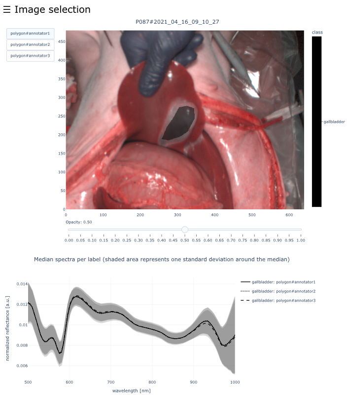
    └── view_organs/  % Interactive visualizations for each image showing the annotated polygons for all annotators and the corresponding median spectra. You can open any document and use the navigation bar to open any image from the dataset
        ├── 01_organ/  % All images which contain this organ (an image may be part of two organ folders if it contains multiple annotated regions)
        │   ├── PXXX#YYYY_MM_DD_HH_MM.html
        │   └── [more images]
        └── [more labels]

Please also have a look at the file reference tutorial which contains detailed information about the different file formats and examples of how to read them in Python.

Frequently Asked Questions

Where can I find the raw spectral data?

The YYYY_MM_DD_HH_MM_SS_SpecCube.dat file (contained within data/subjects/P0xx/YYYY_MM_DD_HH_MM_SS) is the file that contains the raw spectral data with reflectance values for each band and pixel position. Each data cube has the dimensions (480, 640, 100) = (height, width, channels) with the 100 spectral channels being in the range from 500 nm to 1000 nm at a spectral resolution of around 5 nm.

Why are the individual pigs (subjects) named P086 to P096 in the dataset, but not in the figures of the manuscript?

The published data is part of a prospectively growing database for hyperspectral recordings in pigs. In the future, we plan to make more data accessible. In order to allow other research groups to continuously make use of our published datasets and even combine these, it is essential to precisely indicate which datasets have been obtained from which uniquely identifiable animal. In the manuscript and the figures, animals were labeled P01 to P11 in order to avoid confusion for the regular reader. The following table maps each subject identifier from the paper to the subject identifier in the dataset. This table is also provided on the repository website.

subject identifier (manuscript)	subject identifier (dataset)	date of recordings	number of organs recorded	sex
P01	P086	2021_04_15	16	m
P02	P087	2021_04_16	12	f
P03	P088	2021_04_19	17	f
P04	P089	2021_04_21	15	m
P05	P090	2021_04_22	11	f
P06	P091	2021_04_24	7	f
P07	P092	2021_04_27	13	f
P08	P093	2021_04_28	18	f
P09	P094	2021_04_30	19	m
P10	P095	2021_05_02	17	m
P11	P096	2021_05_06	15	m

Do I need licensed software to work with the dataset?

The TIVITA® software is proprietary and especially the underlying formulas for the parameter image computation are unfortunately protected. However, by providing the (numerical) parameter images, extensive interactive visualizations of the data and our code repository, we made sure that the TIVITA® software is not needed for working with our dataset.

What is L1-normalization and why do you use it for all your analysis?

L1-normalization describes a normalization technique that accounts for multiplicative illumination changes arising, for example, from fluctuations in the measurement distance. Given a vector with 100 reflectance values, L1 normalization divides by the L1-norm of the spectra, i.e., the absolute sum of every reflectance value. In Numpy, this can be achieved via

# data.shape = [480, 640, 100]
data = data / np.linalg.norm(data, ord=1, axis=-1, keepdims=True)
data = np.nan_to_num(data, copy=False)

As a consequence, the sum of absolute values for each spectrum will be 1 after this operation. Please note that negative reflectance values are possible due to white and dark calibration. Normalization is crucial when working with spectral data as it can eliminate unwanted differences and shift the focus on important aspects. We demonstrate in the paper that only with normalization the measured reflectance values are comparable to spectrometer measurements (which are the gold standard). This is why we exclusively perform our analyses with normalized data. Preprocessed normalized data for every HSI cube is stored in intermediates/preprocessing/L1.

Why are the L1 preprocessed cubes stored in float16 instead of float32?

The intermediates folder is optimized towards fast data loading for deep learning applications. For this, it is crucial to load the raw data as fast as possible. float16 significantly reduces the file size while we found the loss in precision to be neglectable (detailed precision analysis can be found in this notebook). Please note that it is still possible to cast the data to float32 after loading to increase precision for subsequent operations.

What do the index values StO2, NIR, THI, TWI, OHI and TLI mean?

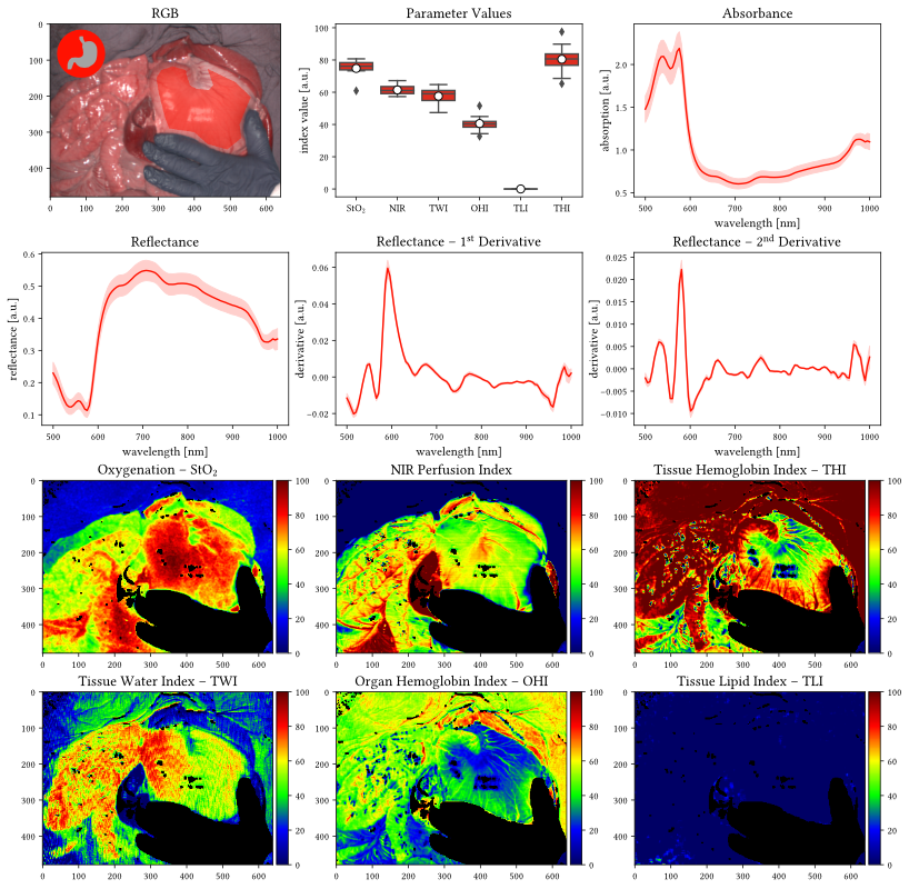
The color-coded indexes were developed and published by the scientific employees of the HSI camera manufacturer Diaspective Vision in the article Hyperspectral imaging in perfusion and wound diagnostics – methods and algorithms for the determination of tissue parameters. The parameter details are confidential, but will be shared by the manufacturer upon reasonable request after signing a non-disclosure agreement.

Tissue oxygenation index (StO2): oxygen saturation of the tissue microcirculatory system
Near-infrared perfusion index (NIR): perfusion of deeper tissue regions (up to several mms) which depends both on the oxygen saturation as well as the hemoglobin distribution.
Tissue hemoglobin index (THI): amount of hemoglobin distributed in the tissue; specifically designed for skin tissue.
Tissue water index (TWI): amount of water present in the tissue.
Organ hemoglobin index (OHI): amount of hemoglobin distributed in the tissue; specifically designed for organ tissue and linearly related to the THI.
Tissue lipid index (TLI): amount of lipids in the tissue.

Where do I find the index values (StO2, NIR, THI, TWI, OHI and TLI) of each recording in the dataset?

The color-coded index images can be found in the image folders in: data/subjects/P0XX/YYYY_MM_DD_HH_MM_SS. The raw data of the computed values can be found in: intermediates/preprocessing/parameter_images

How was the absorbance estimated?

The absorbance was approximated through the negative natural logarithm of the reflectance values based on the modified Beer-Lambert law.

How are RGB images reconstructed from the HSI data?

RGB images are reconstructed from the HSI data by aggregating the spectral channels in the ranges of 530–560 nm, 540–590 nm, and 585–725 nm for blue, green and red, respectively.

Why was the data of 8 pigs per organ not provided from 8 pigs only, but 11 pigs in total?

As depicted transparently in Figure 3 of the paper, for each organ, annotations from 8 pigs are provided. However, these are not necessarily the same 8 pigs. This is due to several challenges in the pig model (e.g., organ aplasia, organ adhesions from presumably previous trauma, circulation insufficiency after several hours of narcosis, etc.). Our goal was to provide annotations for physiological tissue. Therefore, we did not annotate organs that potentially deviate from a physiological state due to the above-mentioned challenges. Therefore, the 8 pigs per organ are distributed across a total of 11 pigs.

Do all images show physiological organs?

Every annotated region is physiological and this is true for most unannotated regions as well. However, we always design our animal experiments to cover as many studies as possible to limit the total number of animal experiments (3 R’s principles for animal experiments: Replace, Reduce, Refine). For this reason, it is possible that in some images, side effects from other studies are visible. Specifically, the images for the two subjects P086 and P090 listed below do not show physiological kidney due to another study being in preparation at the time of image acquisition. However, the protocol of measuring the physiological organs was compatible.

P086: 2021_04_15_13_39_06, 2021_04_15_13_39_25, 2021_04_15_13_39_41, 2021_04_15_13_40_04, 2021_04_15_13_40_20, 2021_04_15_13_40_37, 2021_04_15_13_41_00, 2021_04_15_13_41_16, 2021_04_15_13_41_32, 2021_04_15_13_42_05, 2021_04_15_13_42_22, 2021_04_15_13_42_38, 2021_04_15_13_43_14, 2021_04_15_13_43_36, 2021_04_15_13_43_52, 2021_04_15_13_44_25, 2021_04_15_13_44_43, 2021_04_15_13_45_00
P090: 2021_04_22_13_04_28, 2021_04_22_13_04_44, 2021_04_22_13_05_01, 2021_04_22_13_05_51, 2021_04_22_13_06_08, 2021_04_22_13_06_25, 2021_04_22_13_07_23, 2021_04_22_13_07_40, 2021_04_22_13_08_00

If you have any additional questions about the dataset or its usage, feel free to head over to https://github.com/IMSY-DKFZ/htc and connect with us 😊 Alternatively, you can contact us at info@heiporspectral.org.

License

This dataset is made available under the Creative Commons Attribution 4.0 International License (CC-BY 4.0). If you whish to use or reference this dataset, please cite our paper “HeiPorSPECTRAL - the Heidelberg Porcine HyperSPECTRAL Imaging Dataset of 20 Physiological Organs”.

Cite via BibTeX

@article{Studier-Fischer2023,
  author={Studier-Fischer, Alexander and Seidlitz, Silvia and Sellner, Jan and Bressan, Marc and Özdemir, Berkin and Ayala, Leonardo and Odenthal, Jan and Knoedler, Samuel and Kowalewski, Karl-Friedrich and Haney, Caelan Max and Salg, Gabriel and Dietrich, Maximilian and Kenngott, Hannes and Gockel, Ines and Hackert, Thilo and Müller-Stich, Beat Peter and Maier-Hein, Lena and Nickel, Felix},
  title={HeiPorSPECTRAL - the Heidelberg Porcine HyperSPECTRAL Imaging Dataset of 20 Physiological Organs},
  journal={Scientific Data},
  year={2023},
  month={Jun},
  day={24},
  volume={10},
  number={1},
  pages={414},
  issn={2052-4463},
  doi={10.1038/s41597-023-02315-8},
  url={https://doi.org/10.1038/s41597-023-02315-8}
}

Neither this website nor any of its subdomains process any user data. No access logs are created. Files are served via the servers of all-inkl.com.

Acknowledgements

We acknowledge the data storage service SDS@hd supported by the Ministry of Science, Research and the Arts Baden-Württemberg (MWK) and the German Research Foundation (DFG) through grant INST 35/1314-1 FUGG and INST 35/1503-1 FUGG. This project has received funding from the European Research Council (ERC) under the European Union’s Horizon 2020 research and innovation programme (NEURAL SPICING, Grant agreement No. 101002198) and was supported by the German Cancer Research Center (DKFZ) and the Helmholtz Association under the joint research school HIDSS4Health (Helmholtz Information and Data Science School for Health). It further received funding from the Surgical Oncology Program of the National Center for Tumor Diseases (NCT) Heidelberg and the structured postdoc program of the NCT.